Parameter Identification

The parameter identification part of Circulatory_Autogen is designed to allow calibration of a model to experimental or clinical data. It implements an optimisation method to find the best fit parameters that give a minimal (local minima) error difference between the model output and the ground truth observables (experimental or clinical data or user specified). The creation of below two configuration files is necessary:

• params_for_id
• param id observables

Those files should be added to the [CA_dir]/resources directory (or your custom resources_dir). Proper names of the files are [file_prefix]_params_for_id.csv and [file_prefix]_obs_data.json, respectively. You can also set params_for_id_file in user_inputs.yaml if you want to use a non-standard filename.

Prerequisites

• A generated model (see Model Generation and Simulation).
• param_id_obs_path and params_for_id files in your resources directory.
• OpenCOR Python environment with MPI if running in parallel.

Creating params_for_id file

This file defines which parameters (constants and initial_states) within your model that you will vary in the parameter id process and their allowed ranges (prior distribution). Following is an example of the params_for_id.csv file.

The entries in the file are detailed as follows:

• vessel_name: the name of the vessel/module the parameter is in
• param_name: the name of the parameter in the cellml module (not including the "vessel_name" suffix that is included in the [file_prefix]_parameters.csv file).
• param_type: "state" or "const"; whether the parameter is the initial value of a state or a const.
• min: The minimimum of the range of possible values (min of the uniform distribution).
• max: The maximum of the range of possible values (max of the uniform distribution).
• name_for_plotting: The name (latex format) that will be used when automatically potting comparisons with observables and predictions.

Note

param_type will be deprecated. All should be "const". Initial values that need to identified should be defined as constants within the cellml module.

Info

In the future we plan on including other types of priors rather than just uniform.

Creating param id observables file

This file defines the simulation protocol (protocol_info), and ground truth observables that will be used in the cost function for the parameter id optimisation algorithm. It also defines the measurement standard deviation, and weighting for each observable.

File path of the obs_data.json file should be defined as param_id_obs_path in [CA_dir]/user_run_files/user_inputs.yaml. This path can be absolute or relative to the location of your user_inputs.yaml.

Note

IMPORTANT: For creating obs_data.json files in python (strongly recommended over modifying the json by hand you can use the helper class in src/utilities/obs_data_helpers.py. See src/scripts/example_format_obs_data_json_file.py for an example that you can copy and change for your parameter identification task.

protocol info

The protocol info defines the numerical experiments you will be running. Here is an example for a sympathetic neuron calibration where the input current is changed from 0 to 0.15 pA after 1 second then simulated for 2 seconds with that input current. This was performed in two experiments, the first experiment with a M-type potassium conductance of 0.08 uS and the second experiment with an increased M-type potassium channel conductance of 0.12 uS.

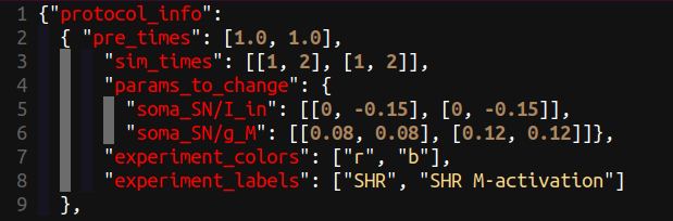
For the protocol we define each experiment as each new full simulation that needs to be run. Each subexperiment is a section of an experiment with its own set of parameters. Subexperiments generally relate to different time periods where the inputs in the experiments that are being used for calibration have a change in value (e.g. change in drug concentration, change in stimulatiion frequency, change in applied force). The entries in the protocol info are:

• pre_times: The amount of simulation that is done before you want to compare to observables or plot (this part of the simulation is thrown away. This is mainly used to simulate for an amout of time to reach steady state or periodic state. shape = (number of experiments)
• offline_pre_time (optional): A single scalar, in seconds. Before any experiment runs, the solver performs one unlogged warmup integration for this duration, then stores the end state as the default state used when reset_states() is called at the start of each experiment. Use this to separate a long steady-state or periodic warmup from the logged pre_times phase. Supported for CVODE_myokit, casadi_python, and python (solve_ivp) backends; not available for OpenCOR. Example: offline_pre_time: 19.0 with pre_times: [1.0] gives 20 s of total warmup before the first logged segment, equivalent to pre_times: [20.0] without offline_pre_time.
• sim_times: The length in time of each subexperiment. shape=(number of experiments, number of subexperiments) -- Note: the shape isn't completely correct here, the number of subexperiments can be different for each experiment
• params_to_change: A dictionary where the key is a parameter name and the entry is the assigned value of that parameter in each (experiment_idx, subexperiment_idx).
• experiment_colors: The line color for the plots of each experiment.
• experiment_labels: The label for each experiment, which is used for plotting and naming plots.

data items

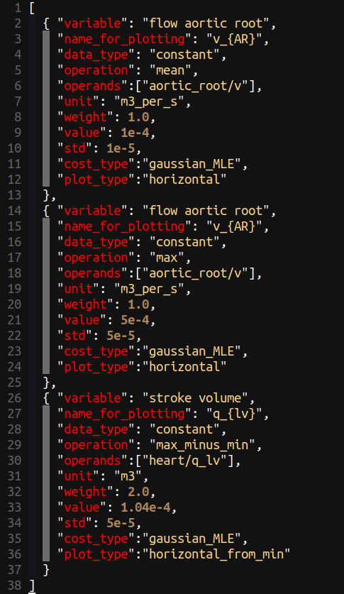
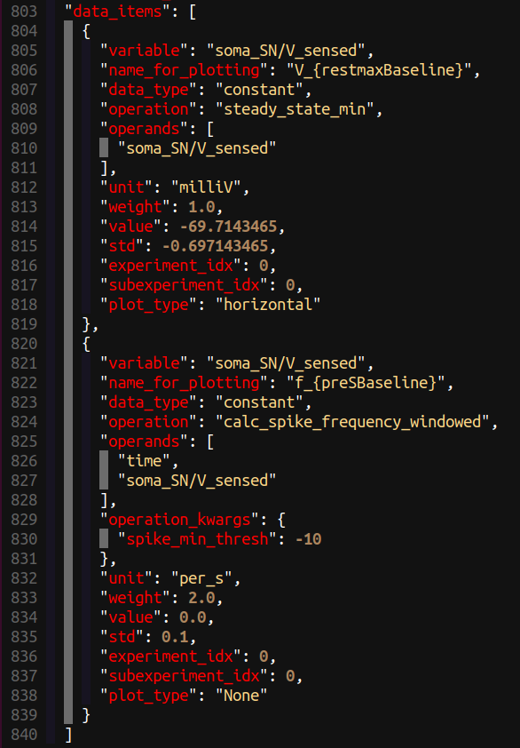
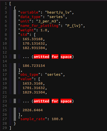
Examples of obs_data.json, data_item entries are shown in below figures for constant, constant with operation_kwargs, series, and frequency data types, respectively.

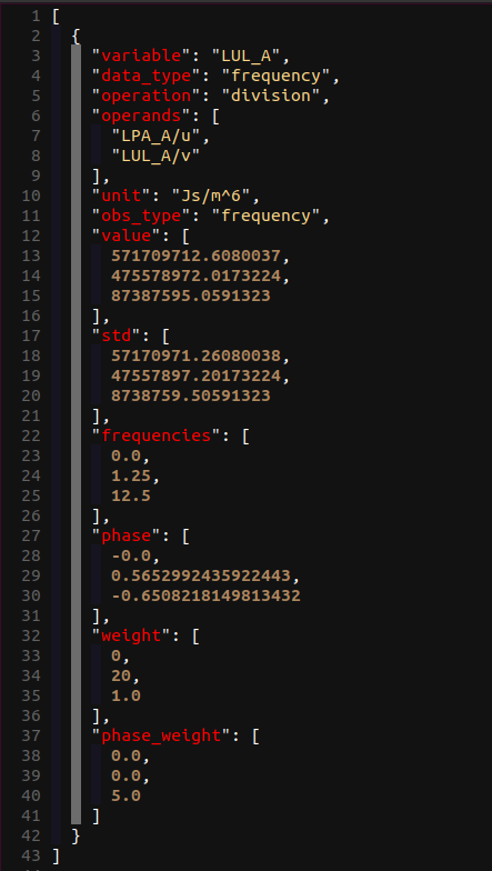
The entries in the data_item list in the obs_data.json file are:

• variable: This is the user defined observable name, it does not need to link to the cellml variable name.
• data_type: The format of the data. This can be "constant", "series", or "frequency" as shown above.
• unit: The unit of the observable.
• name_for_plotting: The name that will be in the automated plots comparing observable data to model output. (latex format)
• weight: The weighting to put on this observables entry in the cost function. Default should be 1.0
• std: The standard deviation which is used in the cost function. The cost function is the relative absolute error (AE) or mean squared error (MRE), each normalised by the std.
• value: The value of the ground truth, either a scalar for constant data_type, or a list of values for series or frequency data_types.
• obs_dt: required for series data types and not needed for constant or frequency. It defines the timestep for the observable series values.

Series ground truth from .npy files (t_path and value_path)

For large time-series observables you can store arrays in NumPy files instead of embedding long lists in the JSON. On load, Circulatory Autogen reads the files and fills in any missing value and obs_dt fields before calibration runs. You must still set std in the JSON (see below).

• t_path: Path to a .npy file containing the time vector (seconds).
• value_path: Path to a .npy file containing the observable values. This is always the quantity that will be compared to the model .

Paths may be absolute or relative to the process working directory when parameter identification is started. If value is already present in the JSON, the file path should not be set;

Example data_item entry:

{
  "variable": "P aortic root",
  "data_type": "series",
  "operands": ["aortic_root/u"],
  "operation": null,
  "unit": "Pa",
  "weight": 1.0,
  "std": 500.0,
  "t_path": "/path/to/pressure_time.npy",
  "value_path": "/path/to/pressure_values.npy",
  "experiment_idx": 0,
  "subexperiment_idx": 0
}

If obs_dt is omitted, it is estimated from the mean step in t_path. For std, provide either one positive number (applied to every sample in the series) or a list with one entry per sample (same length as value after load).

Warning

The dt or sample_rate fields are deprecated for series data. Use obs_dt instead.

Not to be confused with the dt for the model simulation outputs. - operation: This defines the operation that will be done on the operands/variable. The possible operations to be done on model outputs are defined in [CA_dir]/src/param_id/operation_funcs.py and in [CA_dir]/funcs_user/operation_funcs_user.py for user defined operations. - operation_kwargs: This is a dictionary of key word arguments (kwargs) and their values that links to the kwargs in the chosen python operation function. - operands: The above defined "operation" can take in multiple variables. If operands is defined, then the "variable" entry will be a placeholder name for the calculated variable and the operands will define the model variables that are used to calculate the final feature that will be compared to the observable value entry/s. - experiment_idx and subexperiment_idx: Optional indices to link a data item to a specific experiment/subexperiment in protocol_info.

Warning

obs_type: Deprecated in favor of operation.

prediction items (optional)

You can include a prediction_items list in obs_data.json to request additional model outputs to plot (not used in the cost function). Each entry includes:

• variable
• unit
• experiment_idx (optional; defaults to 0)
• name_for_plotting (optional)

Running external cellml models

Running cellml models that weren't generated with Circulatory_Autogen is also just as straightforward:

Simply set the file_prefix in your user_inputs.yaml file to the name of your cellml model <file_prefix>.cellml. Then set generated_models_dir to the path to the dir where your model subdir is and the subdir where the calibrated model will be generated. Make sure your cellml file/files are in a directory of the same name i.e.:

path/to/your/generated_models_dir/<file_prefix>/<file_prefix>.cellml

After calibration, the following directory will be created with your generated model:

path/to/your/generated_models_dir/<file_prefix>_<obs_file_name>/

Note

Currently the generated model needs to be run in newer OpenCOR with the LibOpenCOR backend because a CellML 2.0 model is generated.

Creating your own operations

To enable flexibility we allow you to create your own user-defined operation functions in python to extract features from your model outputs and compare to data in the calibration. Available operation functions can be found in src/param_id/operation_funcs.py and in the file made for adding your own operation functions in funcs_user/operation_funcs_user.py. Here is an example of an operation function for calculating the ratio of the two peaks (used for mitral valve flow).

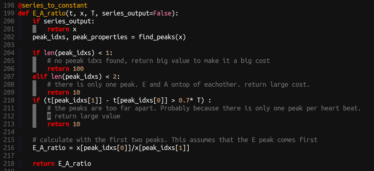
Note:

• kwargs can be used and defined for each entry in your obs_data.json with operation_kwargs, see above.
• if series_output is needed to return the variable trace for plotting.
• A more elegant method of returning a high cost if the observable can't be calculated is being discussed.

Creating your own cost functions

To allow even more flexibility, we also allow users to define their own cost functions (or likelihood functions). These can be found at funcs_user/cost_funcs_user.py. An example for the maximum likelihood estimator for gaussian noise (equivalent to weighted mean squared error) is:

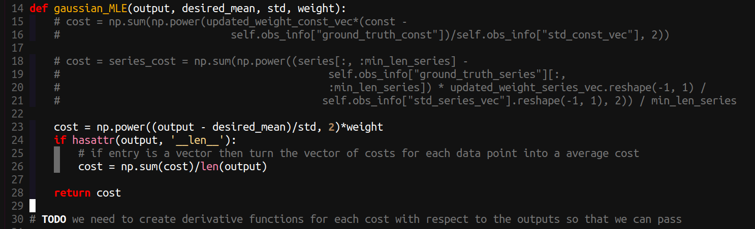
Note:

• Currently there are no kwargs for user defined cost functions. But there will be: see issue

Solver

Before doing calibration, a solver for the model needs to be chosen

• solver defines the solver family. Options depend on model_type:
  • CellML (model_type: cellml_only): CVODE defaults to CVODE_myokit (Myokit). Use CVODE_opencor explicitly if you want the OpenCOR backend instead.
  • Python (model_type: python): solve_ivp with solver_info.method set to RK45, BDF, etc.
  • CasADi Python (model_type: casadi_python): casadi_integrator with solver_info.method set to cvodes, idas, collocation, rk, semi_implicit_euler, or bdf.
  • C++ (model_type: cpp): CVODE, RK4, or PETSC.
• solver_info defines settings for the chosen solver:
  • dt_solver: solver time step (for CVODE this sets MaximumStep when provided)
  • MaximumStep: maximum step size for adaptive solvers
  • MaximumNumberOfSteps: maximum number of substeps before stepping
  • method: any method for solve_ivp or casadi_integrator, e.g. RK45, BDF, cvodes, etc.

Automatic differentiation supports constant and series observables only

With do_ad: true the cost is built symbolically. constant and series data items are both supported, and dt does not have to equal a series item's obs_dt: the simulated series is linearly interpolated onto the observation times, which is a multiply by a matrix of weights fixed by the two time grids, so it stays differentiable. Frequency (amp / phase) and prob_dist observables cannot be differentiated yet, and raise rather than silently contributing nothing to the cost.

CasADi semi_implicit_euler — enables automatic differentiation on stiff models (verify with a convergence study)

When using gradient-based parameter identification (param_id_method: sp_minimize with do_ad: true) on a very stiff model, the adaptive cvodes integrator can solve the forward problem but its adjoint-sensitivity gradient fails (e.g. CasADi raises CVodeF returned "CV_ERR_FAILURE"). The full 3compartment cardiovascular model — whose valve dynamics are extremely stiff and contain discontinuous (floor-driven) heart activation — is a typical case.

For these models set solver_info.method: semi_implicit_euler. This is a fixed-step, linearly-implicit (semi-implicit) Euler scheme with diagonal-Jacobian damping:

x_{n+1} = x_n + dt * f(x_n) / (1 - dt * d f_i / d x_i)

The damping term stabilises the stiff modes at the model dt, and because the whole integrator is built as a single symbolic graph, CasADi differentiates the cost by ordinary reverse-mode AD — there is no adjoint ODE solver to fail. This makes exact gradients (and gradient-based optimisation) available for stiff models where cvodes cannot produce a gradient.

model_type: casadi_python
solver_info:
  solver: casadi_integrator
  method: semi_implicit_euler
  max_step_size: 0.001

Less accurate than cvodes — do a convergence study

semi_implicit_euler is a first-order, fixed-step scheme that damps using only the diagonal of the Jacobian, so it is less accurate than the adaptive cvodes integrator and, on a stiff model, can noticeably differ from the true (CVODE) trajectory at a practical dt. It is provided so that AD gradients are available on stiff models where cvodes cannot produce one — not because it is the accurate choice.

Do not trust the results at a single dt. Perform a convergence study: rerun with progressively smaller dt (e.g. halve it) and confirm the trajectories and the identified parameters stop changing meaningfully before relying on them. Where cvodes works, it remains the more accurate default.

CasADi bdf — a more accurate stiff AD method that also supports a long pre_time

bdf is a fixed-step, symbolic implicit BDF2 scheme (a rootfinder per step, differentiated through the implicit-function theorem). Like semi_implicit_euler it is built as a single symbolic graph, so CasADi produces exact gradients by reverse-mode AD with no adjoint solver to fail — but it is second order and full-Jacobian implicit, so it tracks a stiff trajectory far more accurately than the first-order, diagonally-damped semi_implicit_euler at the same dt. It also handles a nonzero pre_time warmup (unlike cvodes, whose adjoint typically fails with CV_TOO_MUCH_WORK over a long warmup). Prefer bdf over semi_implicit_euler for stiff models; still do a convergence study in dt.

model_type: casadi_python
solver: casadi_integrator
do_ad: true
solver_info:
  method: bdf
  max_step_size: 0.001

Myokit CVODES forward sensitivity — AD gradients for cellml_only models

A cellml_only model run through the Myokit backend can produce an exact gradient without converting to casadi_python, using Myokit's native CVODES forward-sensitivity analysis (FSA). Set model_type: cellml_only, solver: CVODE_myokit, do_ad: true, and a gradient-based param_id_method (sp_minimize or multi_start_sp_minimize). FSA integrates the state and sensitivity equations together with the adaptive stiff CVODES solver, so it handles stiff dynamics and a long pre_time warmup natively while staying as accurate as the forward simulation itself.

model_type: cellml_only
solver: CVODE_myokit
do_ad: true
param_id_method: multi_start_sp_minimize
solver_info:
  rtol: 1e-9
  atol: 1e-9        # tight tolerances keep the sensitivities out of the integrator noise floor

A parameter that only sets a state's initial value cannot be a CVODES sensitivity independent; such parameters automatically fall back to finite differences (a one-line warning reports how many and which). Tighten rtol/atol when using FSA so the sensitivities are well resolved.

our AADC wrapper is not yet suitable for stiff models or multiple observables

The AADC tape backend (model_type: aadc_python) records a fixed-step integrator, which is inaccurate or unstable on stiff models — on the 3compartment cardiovascular model its fixed-step implicit solve deviates from CVODE by orders of magnitude. Every AADC run now probes the first second of dynamics and prints a loud warning if the model is stiff, pointing you at CasADi bdf or Myokit CVODES FSA instead.

AADC is also not currently suitable for problems with multiple observables. Its tape cost can only represent an observable whose operand is a state with a reimplemented operation (max/min/mean), in a single experiment. Any other observable — one whose operand is an algebraic variable (e.g. a pressure or flow computed from the states rather than integrated), an operation the tape does not reimplement (e.g. max_minus_min), or a series/other data type — cannot be put on the tape. Rather than silently minimise a reduced cost over only the tapeable subset (which would give a fit that is wrong for the omitted observables), the AADC gradient path raises an error as soon as any observable in the set can't be taped, naming the offending observables and pointing at the tracking issue (#258). On the 3compartment model, for instance, only 2 of the 6 observables are tapeable (the aortic_root/u features are algebraic and heart/q_lv uses max_minus_min), so AADC refuses to run there and is left off that benchmark. Full-cost parity needs the algebraic variables recomputed on the tape from the state trajectory and max_minus_min support (tracked in issue #258). Until then, use AADC only for non-stiff, single-experiment problems whose observables are all state-operand max/min/mean features (or state series); for other observables use casadi_python (method: bdf) or a Myokit CVODES FSA run, which the error message also points you to. Future work will get it working for stiff models and general observables so its advantages for large numbers of parameters can be used.

Multiple sub-experiments / experiments are not yet supported by the AADC wrapper. The tape records one straight-line integration, so a protocol with more than one sub-experiment (or more than one experiment) raises rather than silently differentiating the wrong thing. The Myokit CVODES FSA gradient (model_type: cellml_only + solver: CVODE_myokit) does support multi-sub protocols; the AADC equivalent is tracked as future work.

Parameter Identification Settings

To run the parameter identification we need to set a few entries in the [CA_dir]/user_run_files/user_inputs.yaml file:

• param_id_method: this defines the optimisation method we use. Currently supported methods are:
  • genetic_algorithm: Genetic algorithm optimizer (default, well-tested)
  • CMA-ES: Covariance Matrix Adaptation Evolution Strategy using Nevergrad (supports parallel execution)
  • bayesian: Bayesian optimization using scikit-optimize (deprecated, untested)
  • sp_minimize: Gradient-based optimizer (L-BFGS-B, local only)
  • multi_start_sp_minimize: Multi-start L-BFGS-B — a gradient-based descent from many scattered starting points, so it exploits the gradient but still escapes local minima
• pre_time: this is the amount of time the simulation is run to get to steady state before comparing to the observables from obs_data.json. IMPORTANT: THis is overwritten by the pre_times within the obs_data.json file, see the next section.
• sim_time: The amount of time used to compare simulation output and observable data. This should be equal to the length of a series observable entry divided by the "sample_rate". If not, only up to the minimum length of observable data and modelled data will be compared.
• dt: The output (sample) time step for model outputs
• solver_info.dt_solver: The solver time step for CVODE (sets MaximumStep when provided)
• solver_info.MaximumStep: The CVODE maximum step size if dt_solver is not provided
• param_id_obs_path: the path to the obs_data.json file described above (absolute or relative to your user_inputs.yaml).
• ga_options: Legacy dictionary (deprecated, use optimiser_options instead):
  • cost_type: "AE" or "MSE" for absolute error or mean squared error.
  • num_calls_to_function: How many forward simulations of pre_time+sim_time will be run in the optimisation algorithm.
  • cost_convergence: If the cost value is lower than this threshold then the calibration run is complete.
  • max_patience: If the cost doesn't improve for this number of simulations, then calibration is complete (we assume that the cost has converged to the global minima or can't get out of a local minima).

• Note: For backwards compatibility, entries in ga_options are automatically merged into optimiser_options if not already present. It is recommended to use optimiser_options instead.

• optimiser_options: Dictionary for optimizer-specific options (preferred over ga_options). Common options shared across optimisers:

  • num_calls_to_function: Maximum number of function evaluations (default: 10000)
  • cost_convergence: Convergence tolerance for cost (default: 0.0001)
  • max_patience: Maximum patience for convergence (default: 10)
  • cost_type: Cost function type (e.g., 'MSE')

  CMA-ES specific options:

  • sigma0: Initial standard deviation for CMA-ES (optional, default: 0.2 of parameter range)
  • Note:
    • The number of parallel workers is automatically determined from the number of MPI processes
    • Initial parameter values are automatically loaded from {file_prefix}_parameters.csv

  sp_minimize specific options:

  • do_ad: Boolean value to determine whether to use automatic differentiation for gradient calculation. If it's set to False, gradients will be estimated using finite difference approximation.

  multi_start_sp_minimize specific options:

  • num_starts: Number of L-BFGS-B descents to run (default: 10, or 4 when DEBUG is true). The starts are spread round-robin over the MPI ranks; make num_starts several times the rank count so the work balances (see the note under "Multi-start Gradient-based Optimizer" below).
  • start_sampling: How the starting points are scattered over the parameter bounds: sobol (default), latin_hypercube or random.
  • include_init_point: If true (default), the first start is the initial parameter values from {file_prefix}_parameters.csv, so this method can never do worse than a single-start sp_minimize run.
  • seed: Seed for the start sampler (default: 0), so a run is repeatable.
  • fd_step: Finite-difference step used when an automatic-differentiation gradient isn't available — i.e. any configuration without an AD backend (see the gradient-backend note below), or when do_ad: false (default: 1e-4).
  • cost_convergence: Once any start reaches this cost, every MPI rank stops launching new starts (signalled between ranks with a non-blocking message), so no rank keeps working after a good-enough solution has been found. (Set no_new_starts_on_convergence: false to disable this.)
  • no_new_starts_on_convergence: true (default) is the behaviour above — stop launching starts once one converges. Set to false to run every start regardless, then report how many converged and how many landed in each distinct minimum. That maps the basin structure of a multi-modal problem (which minima exist, and how the starts split between them); the counts are written to multi_start_convergence_clusters.csv and printed at the end of the run.
  • convergence_cluster_tol_frac: When counting how many starts reached each minimum, two converged starts are treated as the same solution if every parameter agrees to within this fraction of that parameter's range (default: 0.02, i.e. 2%).

  Automatic-differentiation gradient backends

  Gradient-based calibration (do_ad: true) is provided by two open-source backends: CasADi (model_type: casadi_python, LGPL — symbolic differentiation) and Myokit CVODES forward sensitivity (model_type: cellml_only + solver: CVODE_myokit). Both require no proprietary licence and both handle stiff models; see the Solver section for which method to pick.

  Circulatory Autogen also ships an optional adapter for AADC (Matlogica), which is third-party proprietary software, not part of Circulatory Autogen, not bundled with it, and restricted to academic/non-commercial use under Matlogica's own licence. It is not required. It can drive sp_minimize / multi_start_sp_minimize only for non-stiff, state-observable, single-experiment problems (its tape records a fixed-step integrator); it is unsuitable for stiff models such as the full cardiovascular model. See Optional third-party backends if you already hold a Matlogica licence.

• ga_options: Legacy dictionary for optimization options. For backwards compatibility, entries in ga_options are automatically merged into optimiser_options if not already present. It is recommended to use optimiser_options instead.

Choosing an Optimization Method

Genetic Algorithm (genetic_algorithm)

• Pros: Well-tested, robust, handles non-smooth cost functions well
• Cons: Can be slower, requires more function evaluations
• Best for: Complex, multi-modal optimization problems, when you have many function evaluations available

CMA-ES (CMA-ES)

• Pros: Efficient gradient-free optimization, supports parallel execution, good convergence properties
• Cons: Requires Nevergrad package (pip install nevergrad)
• Best for: Smooth optimization landscapes, when you want faster convergence with parallel execution

Example configuration for CMA-ES:

param_id_method: CMA-ES
optimiser_options:
  num_calls_to_function: 10000  # shared option
  cost_convergence: 0.001         # shared option
  sigma0: 0.1                      # CMA-ES specific (optional, initial standard deviation)
  # Note: Initial parameter values are automatically loaded from {file_prefix}_parameters.csv

Gradient-based Optimizer (sp_minimize)

• Pros: Efficient gradient-based optimization, fast convergence
• Cons: Can get stuck in local minima
• Best for: Smooth optimization landscapes, when you want faster convergence

For an AD gradient use model_type: casadi_python (CasADi symbolic differentiation) or a cellml_only model run through solver: CVODE_myokit with do_ad: true (Myokit CVODES forward sensitivity — see the Solver section). Any other configuration falls back to a finite-difference gradient.

Multi-start Gradient-based Optimizer (multi_start_sp_minimize)

L-BFGS-B only ever finds the minimum of the basin it starts in, so on a multi-modal cost surface sp_minimize is at the mercy of the initial parameter values. This method scatters num_starts starting points over the parameter bounds and runs a bounded L-BFGS-B descent from each one, keeping the best minimum found. It explores globally, like the population-based optimisers, while still using the gradient to descend each basin quickly and accurately.

• Pros: Escapes local minima while still exploiting the gradient; the starts are independent so they are distributed over the MPI ranks with no communication; typically reaches a far lower cost than a gradient-free global search for the same wall-clock time.
• Cons: Cost scales with num_starts; a very rugged surface may need many starts.
• Best for: Multi-modal cost surfaces — the common case when calibrating oscillatory models, where a wrong rate constant puts the simulation out of phase with the data.

Parallel multi-start pays off only for many starts

The starts are distributed statically round-robin over the MPI ranks (run_param_id.sh with num_processors > 1). Because individual L-BFGS-B descents vary a lot in length — some converge in a handful of iterations, some take many — the per-rank workloads only even out when each rank runs many starts, i.e. when num_starts is much larger than the number of ranks. With num_starts ≤ num_processors each rank runs a single descent and the wall-clock is bounded by the slowest one, so extra ranks buy little. As a rule of thumb, run with several times as many starts as ranks. Measured on a 20-core host with 100 starts: ~3.8× on 4 ranks, ~4× on 8. Once any start reaches cost_convergence, every rank stops launching new starts, so a converged run doesn't keep the other ranks busy needlessly. run() reports the achieved speedup in its final log line.

This works for any model_type. The gradient comes from get_gradient(), which has an AD backend for casadi_python (symbolic jacobian), cellml_only run through CVODE_myokit with do_ad: true (Myokit CVODES forward sensitivity), and aadc_python (tape reverse pass — non-stiff, state-observable, single-experiment problems only; see the AADC caveat in the Solver section). For every other configuration there is no AD gradient, so the cost is evaluated with the usual simulation cost and the gradient falls back to finite differences.

Example configuration:

param_id_method: multi_start_sp_minimize
model_type: casadi_python     # for AD gradients; other model types use finite differences
solver: casadi_integrator
do_ad: true
optimiser_options:
  cost_convergence: 0.0001
  num_starts: 10              # number of L-BFGS-B descents
  start_sampling: sobol       # sobol | latin_hypercube | random
  include_init_point: true    # first start is the x0 from {file_prefix}_parameters.csv
  seed: 0

Alongside the usual best_cost_history.csv / best_param_vals_history.csv (written as a running-best curve over the concatenated starts), this optimiser writes a multi_start_summary.csv with one row per start — its initial cost, final cost, iteration count and final parameter values. That tells you how many distinct basins your starts fell into, which is the quickest way to see whether num_starts is high enough.

It also streams three live per-start histories during the run, appended one row per L-BFGS-B iteration (iteration 0 is the start point), independent of DEBUG: multi_start_cost_history.csv (start_idx, iteration, cost), multi_start_param_vals_history.csv (start_idx, iteration, then one named column per parameter, holding the actual parameter values — same columns as multi_start_summary.csv) and multi_start_gradient_history.csv (start_idx, iteration, then one named column per parameter, holding the cost gradient dJ/dp in real parameter space at that iterate). Group by start_idx and order by iteration to plot a cost-, parameter- and gradient-vs-iteration line per start while the run is still going. The three files share the same (start_idx, iteration) keys, and start_idx is a stable global index, so rows from starts running concurrently on different MPI ranks demux cleanly regardless of interleaving.

Benchmark: FitzHugh-Nagumo

resources/FitzHugh_Nagumo_* is a deliberately multi-modal benchmark. The FitzHugh-Nagumo excitable-cell model

$$\dot V = c\left(V - \tfrac{V^3}{3} + R\right), \qquad \dot R = -\tfrac{1}{c}\left(V - a + bR\right)$$

is a standard hard case for parameter estimation: its least-squares surface has many local minima, because a wrong recovery rate c puts the simulated spike train out of phase with the data (Ramsay et al. 2007, J. R. Statist. Soc. B 69(5), "Parameter estimation for differential equations: a generalized smoothing approach"). The supplied FitzHugh_Nagumo_parameters.csv starts at (a, b, c) = (0.8, 0.9, 2.0), which sits inside a local basin; the true values are (0.2, 0.2, 3.0).

sp_minimize never leaves the basin it starts in. The genetic algorithm escapes it but, being gradient-free, converges slowly. The multi-start finds the global basin and refines it with the gradient — whatever gradient backend drives it (finite differences, CasADi AD, or Myokit CVODES FSA). The table below is regenerated by the benchmark runner (python benchmarks/run_benchmarks.py --update-docs) and by the Benchmarks GitHub Actions workflow, so the published numbers stay current; they depend on the hardware and MPI rank count used.

Generated by benchmarks/run_benchmarks.py --scaling; wall-clock times depend on the hardware.

FitzHugh-Nagumo (non-stiff, multi-modal)

Gradient-free global searches (genetic algorithm, CMA-ES) vs multi-start L-BFGS-B driven by four gradient sources. Holding the optimiser fixed and varying only the gradient isolates what the gradient buys.

cores: 1, 2, 4, 8; wall-clock seconds per core count; best cost / max param err from the 1-core run (same work is run at every core count).

method	best cost	max param err	1 core (s)	2 cores (s)	4 cores (s)	8 cores (s)
genetic_algorithm	1.6932e-03	0.0036	651.7	363.7	252.5	360.8
CMA-ES	1.4413e+02	0.9265	19.3	14.3	8.5	15.3
multi_start (FD)	2.5232e-03	0.0086	86.8	46.8	51.7	55.0
multi_start (CasADi AD)	3.9704e-06	0.0006	80.9	45.5	52.8	54.6
multi_start (Myokit FSA)	3.8261e-06	0.0006	12.5	6.6	8.1	7.3
multi_start (AADC AD)	1.3751e-06	0.0002	3.9	2.2	3.4	3.8

True parameters: a=0.2, b=0.2, c=3.

3compartment cardiovascular (stiff, 20 s warmup)

Gradient-free global searches vs multi-start L-BFGS-B with the two stiff-capable gradient backends. AADC is not run on this stiff model.

cores: 1, 2, 4, 8; wall-clock seconds per core count; best cost / max param err from the 1-core run (same work is run at every core count).

method	best cost	1 core (s)	2 cores (s)	4 cores (s)	8 cores (s)
genetic_algorithm	2.4738e-02	841.0	428.7	261.3	237.9
CMA-ES	3.2210e-02	38.1	88.9	12.2	11.3
multi_start (Myokit FSA)	2.2553e-02	1946.6	1072.9	726.3	478.8
multi_start (CasADi bdf)	2.2753e-02	858.4	476.2	332.8	339.0
multi_start (AADC AD)	skipped — AADC's tape cost covers only state-operand observables with a reimplemented op (max/min/mean); 3compartment's algebraic-variable observables (aortic_root/u) and its max_minus_min are dropped, so AADC would optimise a reduced cost, not the full one -- excluded until it can replicate the same cost (upstream issue #258)

Goodwin oscillator (external PMR CellML, non-stiff, multimodal)

Gradient-free global searches (genetic algorithm, CMA-ES) vs multi-start L-BFGS-B (finite differences and Myokit CVODES FSA) recovering rate constants of the Goodwin 1965 oscillator, taken directly from the Physiome Model Repository as external CellML. Oscillatory dynamics make the least-squares surface multimodal.

cores: 1, 2, 4, 8; wall-clock seconds per core count; best cost / max param err from the 1-core run (same work is run at every core count).

method	best cost	max param err	1 core (s)	2 cores (s)	4 cores (s)	8 cores (s)
genetic_algorithm	2.2272e-03	1.6251	43.3	23.8	16.1	18.3
CMA-ES	1.5822e-04	0.9326	32.7	1.2	24.9	57.1
multi_start (FD)	9.1452e-15	0.0000	12.5	7.0	4.7	4.6
multi_start (Myokit FSA)	1.5193e-13	0.0000	10.3	7.5	6.1	5.7

True parameters: a_i=72, b_i=2, A_i=36.

The stiff 3compartment cardiovascular benchmark (long warmup, Myokit/CasADi — no OpenCOR needed) runs in the same set; it is slower, so the workflow schedule is weekly. See benchmarks/README.md.

Note: For backwards compatibility, ga_options can still be used and will be automatically merged into optimiser_options.

Running parameter identification

After creating the params_for_id file and the param id observables file, and configuring the above settings, run the parameter identification using the below command.

./run_param_id.sh <NUM_CORES>

Following a successful parameter id process, the model with updated parameters can be generated with:

./run_autogeneration_with_id_params.sh

Note

IMPORTANT: After running the calibration, you should plot the simulation outputs vs the ground truth to analyse the fits!! This can be done with:

./plot_param_id.sh

The generated models will be saved in generated_models/ and plots will be saved in param_id_output/.

Full model time-series dumps (all states and variables) are written as NumPy archives in the param_id output directory:

• all_outputs_with_best_param_vals_exp_{i}.npz — written when calibration completes successfully.
• all_outputs_with_best_param_vals_exp_{i}_plot.npz — written at the start of every plot_outputs() call. Use these to recover trajectories after an interrupted run as long as best_param_vals.npy exists in the same output folder.

If you already have a model and do not want to run autogeneration, use:

./run_param_id_without_autogen.sh <NUM_CORES>

Expected outcome

You should have a calibrated model in generated_models/[file_prefix]_[obs_file_name]/ and plots in param_id_output/.

Troubleshooting

• If you see params_for_id_path ... does not exist, confirm params_for_id_file or file_prefix and your resources_dir.
• If you see obs_dt is required for series entries, add obs_dt to each series data item in obs_data.json.
• If MPI errors occur, ensure OpenMPI/MPICH is installed and mpi4py is available in the OpenCOR environment.